Realistic lightcurves of ellipsoids
This notebook demonstrates how to generate lightcurves within sorcha, under the assumption that the Solar System Objects (SSOs) are simple tri-axial ellipsoids, defined by $ a \ge `b :nbsphinx-math:ge `c$, in simple short-axis rotation mode.
Compared to the Ellipsoidal_Lightcurve model, the projected surface of the ellipsoid accounts for the non-illuminated part.
[1]:
import numpy as np
import pandas as pd

import rocks
import requests

import astropy.units as u
from astropy.coordinates import SkyCoord

from sorcha.modules.PPCalculateApparentMagnitudeInFilter import (
    PPCalculateApparentMagnitudeInFilter,
)

import matplotlib.pyplot as plt

# Constants
au = 1.495978707e8  # AU in km
c = 299792458  # m/s
c_AUperDay = c * (1000 / au) * 86400.0
/home/bcarry/anaconda3/envs/sorcha/lib/python3.11/site-packages/assist/__init__.py:44: UserWarning: pkg_resources is deprecated as an API. See https://setuptools.pypa.io/en/latest/pkg_resources.html. The pkg_resources package is slated for removal as early as 2025-11-30. Refrain from using this package or pin to Setuptools<81.
  import pkg_resources
Lightweight ephemeris function
We will need to compute ephemerides, so let’s query the Miriade Virtual Observatory Web service.
[2]:
def ephemcc(ident, ep, nbd=None, step=None, observer="500", rplane="1", tcoor=5, output=None):
    """Gets asteroid ephemerides from IMCCE Miriade for a suite of JD for a single SSO
    Original function by M. Mahlke

    :ident: int, float, str - asteroid identifier
    :ep: float, str, list - Epoch of computation
    :observer: str - IAU Obs code - default to geocenter: https://minorplanetcenter.net//iau/lists/ObsCodesF.html
    :returns: pd.DataFrame - Input dataframe with ephemerides columns appended
              False - If query failed somehow

    """

    # ------
    # Miriade URL
    url = "https://ssp.imcce.fr/webservices/miriade/api/ephemcc.php"

    # Query parameters
    params = {
        "-name": f"{ident}",
        "-mime": "json",
        "-rplane": rplane,
        "-tcoor": tcoor,
        "-output": "--jd",
        "-observer": observer,
        "-tscale": "UTC",
    }

    if "output" in locals():
        params["-output"] += "," + output

    # Single epoch of computation
    if type(ep) != list:
        # Set parameters
        params["-ep"] = ep
        if nbd != None:
            params["-nbd"] = nbd
        if step != None:
            params["-step"] = step

        # Execute query
        try:
            r = requests.post(url, params=params, timeout=80)
        except requests.exceptions.ReadTimeout:
            return False

    # Multiple epochs of computation
    else:
        # Epochs of computation
        files = {"epochs": ("epochs", "\n".join(["%.6f" % epoch for epoch in ep]))}

        # Execute query
        try:
            r = requests.post(url, params=params, files=files, timeout=50)
        except requests.exceptions.ReadTimeout:
            return False

    j = r.json()

    # Read JSON response
    try:
        ephem = pd.DataFrame.from_dict(j["data"])
    except KeyError:
        return False

    return ephem
Definition of simulation
We first define the epochs of the simulation: starting date (expressed in JD), the number of epochs to simulate, and time step between each (in days).
[3]:
# Choice of time frame
jd0 = 2461041.5  # Start date: here set to 2026-01-01
nbd = 1500  # Number of epochs
step = 0.3  # Time step between epochs (days)
We then define the target. It can be an asteroid name/designation or number. The absolute magnitude and spin properties (coordinates and period) are then retrieved from SsODNet (see Berthier et al., 2023). Alternatively, you can define all parameters by hand:
Hthe absolute magnitudera0the right ascension of the spin coordinates (equatorial frame, in degrees)dec0the declination of the spin coordinates (equatorial frame, in degrees)periodthe sidereal rotation period (in hour)G1andG2the phase curve coefficientsa_bthe ratio of equatorial diameters (a and b)a_cthe ratio between the longest (equatorial) diameter (a) and the polar diameter (c)
[4]:
# Target
sso = 22

# Retrieve the target properties from SsODNet
sc = rocks.Rock(sso)
H = sc.H.value
ra0 = sc.spin.RA0.value
dec0 = sc.spin.DEC0.value
period = sc.spin.period.value[0] / 24.0

# Arbitrary phase function and shape
G1 = 0.62
G2 = 0.14
a_b = 1.5
a_c = 2.0
[5]:
# Generate ephemerides
# We use here a special output from Miriade, dedicated to this kind of photometric modeling
eph = ephemcc(
    sso,
    ep=jd0,
    nbd=nbd,
    step=step,
    tcoor=5,
    observer="X05",
    output="-- iofile(ephemcc-photom.xml),--lighttime",
)
[6]:
# Build the observations dataframe
observations_df = pd.DataFrame(
    {
        "fieldMJD_TAI": eph.Date.values,
        "H_filter": H * np.ones(nbd),
        "G1": G1 * np.ones(nbd),
        "G2": G2 * np.ones(nbd),
        "RA_deg": eph.RA.values,
        "Dec_deg": eph.DEC.values,
        "RA_s_deg": eph.RA_h.values,
        "Dec_s_deg": eph.DEC_h.values,
        "Period": period * np.ones(nbd),
        "Time0": jd0 * np.ones(nbd),
        "phi0": np.radians(0) * np.ones(nbd),
        "RA0": np.radians(ra0) * np.ones(nbd),
        "Dec0": np.radians(dec0) * np.ones(nbd),
        "Period": period * np.ones(nbd),
        "a/b": a_b * np.ones(nbd),
        "a/c": a_c * np.ones(nbd),
        "Range_LTC_km": eph.Dobs.values * au,
        "Obj_Sun_LTC_km": eph.Dhelio.values * au,
        "phase_deg": eph.Phase.values,
    }
)

observations_df
[6]:
| fieldMJD_TAI | H_filter | G1 | G2 | RA_deg | Dec_deg | RA_s_deg | Dec_s_deg | Period | Time0 | phi0 | RA0 | Dec0 | a/b | a/c | Range_LTC_km | Obj_Sun_LTC_km | phase_deg | |
|---|---|---|---|---|---|---|---|---|---|---|---|---|---|---|---|---|---|---|
| 0 | 2461041.5 | 6.79 | 0.62 | 0.14 | 359.334334 | -11.523769 | 18.478296 | -3.665327 | 0.172842 | 2461041.5 | 0.0 | 3.405137 | -0.049463 | 1.5 | 2.0 | 4.177865e+08 | 4.049300e+08 | 20.522908 |
| 1 | 2461041.8 | 6.79 | 0.62 | 0.14 | 359.407445 | -11.465113 | 18.536963 | -3.629770 | 0.172842 | 2461041.5 | 0.0 | 3.405137 | -0.049463 | 1.5 | 2.0 | 4.183388e+08 | 4.048958e+08 | 20.502883 |
| 2 | 2461042.1 | 6.79 | 0.62 | 0.14 | 359.482166 | -11.406700 | 18.595636 | -3.594204 | 0.172842 | 2461041.5 | 0.0 | 3.405137 | -0.049463 | 1.5 | 2.0 | 4.188799e+08 | 4.048617e+08 | 20.481478 |
| 3 | 2461042.4 | 6.79 | 0.62 | 0.14 | 359.555298 | -11.348389 | 18.654314 | -3.558628 | 0.172842 | 2461041.5 | 0.0 | 3.405137 | -0.049463 | 1.5 | 2.0 | 4.194149e+08 | 4.048277e+08 | 20.461570 |
| 4 | 2461042.7 | 6.79 | 0.62 | 0.14 | 359.628519 | -11.289645 | 18.712998 | -3.523043 | 0.172842 | 2461041.5 | 0.0 | 3.405137 | -0.049463 | 1.5 | 2.0 | 4.199635e+08 | 4.047937e+08 | 20.441432 |
| ... | ... | ... | ... | ... | ... | ... | ... | ... | ... | ... | ... | ... | ... | ... | ... | ... | ... | ... |
| 1495 | 2461490.0 | 6.79 | 0.62 | 0.14 | 100.442283 | 35.559274 | 125.440170 | 30.992455 | 0.172842 | 2461041.5 | 0.0 | 3.405137 | -0.049463 | 1.5 | 2.0 | 3.696081e+08 | 4.089152e+08 | 21.330520 |
| 1496 | 2461490.3 | 6.79 | 0.62 | 0.14 | 100.514005 | 35.545997 | 125.518137 | 30.985766 | 0.172842 | 2461041.5 | 0.0 | 3.405137 | -0.049463 | 1.5 | 2.0 | 3.702196e+08 | 4.089530e+08 | 21.336566 |
| 1497 | 2461490.6 | 6.79 | 0.62 | 0.14 | 100.583783 | 35.532027 | 125.596080 | 30.979031 | 0.172842 | 2461041.5 | 0.0 | 3.405137 | -0.049463 | 1.5 | 2.0 | 3.708370e+08 | 4.089908e+08 | 21.344123 |
| 1498 | 2461490.9 | 6.79 | 0.62 | 0.14 | 100.656047 | 35.517137 | 125.673996 | 30.972250 | 0.172842 | 2461041.5 | 0.0 | 3.405137 | -0.049463 | 1.5 | 2.0 | 3.714625e+08 | 4.090287e+08 | 21.349582 |
| 1499 | 2461491.2 | 6.79 | 0.62 | 0.14 | 100.729880 | 35.503386 | 125.751888 | 30.965424 | 0.172842 | 2461041.5 | 0.0 | 3.405137 | -0.049463 | 1.5 | 2.0 | 3.720775e+08 | 4.090665e+08 | 21.353868 |
1500 rows × 18 columns
[7]:
# Build the observations dataframe
observations_df = pd.DataFrame(
    {
        "fieldMJD_TAI": eph.Date.values,
        "H_filter": H * np.ones(nbd),
        "G1": G1 * np.ones(nbd),
        "G2": G2 * np.ones(nbd),
        "RA_deg": eph.RA.values,
        "Dec_deg": eph.DEC.values,
        "RA_s_deg": eph.RA_h.values,
        "Dec_s_deg": eph.DEC_h.values,
        "Period": period * np.ones(nbd),
        "Time0": jd0 * np.ones(nbd),
        "phi0": np.radians(0) * np.ones(nbd),
        "RA0": np.radians(ra0) * np.ones(nbd),
        "Dec0": np.radians(dec0) * np.ones(nbd),
        "Period": period * np.ones(nbd),
        "a/b": a_b * np.ones(nbd),
        "a/c": a_c * np.ones(nbd),
        "Range_LTC_km": eph.Dobs.values * au,
        "Obj_Sun_LTC_km": eph.Dhelio.values * au,
        "phase_deg": eph.Phase.values,
    }
)

observations_df
[7]:
| fieldMJD_TAI | H_filter | G1 | G2 | RA_deg | Dec_deg | RA_s_deg | Dec_s_deg | Period | Time0 | phi0 | RA0 | Dec0 | a/b | a/c | Range_LTC_km | Obj_Sun_LTC_km | phase_deg | |
|---|---|---|---|---|---|---|---|---|---|---|---|---|---|---|---|---|---|---|
| 0 | 2461041.5 | 6.79 | 0.62 | 0.14 | 359.334334 | -11.523769 | 18.478296 | -3.665327 | 0.172842 | 2461041.5 | 0.0 | 3.405137 | -0.049463 | 1.5 | 2.0 | 4.177865e+08 | 4.049300e+08 | 20.522908 |
| 1 | 2461041.8 | 6.79 | 0.62 | 0.14 | 359.407445 | -11.465113 | 18.536963 | -3.629770 | 0.172842 | 2461041.5 | 0.0 | 3.405137 | -0.049463 | 1.5 | 2.0 | 4.183388e+08 | 4.048958e+08 | 20.502883 |
| 2 | 2461042.1 | 6.79 | 0.62 | 0.14 | 359.482166 | -11.406700 | 18.595636 | -3.594204 | 0.172842 | 2461041.5 | 0.0 | 3.405137 | -0.049463 | 1.5 | 2.0 | 4.188799e+08 | 4.048617e+08 | 20.481478 |
| 3 | 2461042.4 | 6.79 | 0.62 | 0.14 | 359.555298 | -11.348389 | 18.654314 | -3.558628 | 0.172842 | 2461041.5 | 0.0 | 3.405137 | -0.049463 | 1.5 | 2.0 | 4.194149e+08 | 4.048277e+08 | 20.461570 |
| 4 | 2461042.7 | 6.79 | 0.62 | 0.14 | 359.628519 | -11.289645 | 18.712998 | -3.523043 | 0.172842 | 2461041.5 | 0.0 | 3.405137 | -0.049463 | 1.5 | 2.0 | 4.199635e+08 | 4.047937e+08 | 20.441432 |
| ... | ... | ... | ... | ... | ... | ... | ... | ... | ... | ... | ... | ... | ... | ... | ... | ... | ... | ... |
| 1495 | 2461490.0 | 6.79 | 0.62 | 0.14 | 100.442283 | 35.559274 | 125.440170 | 30.992455 | 0.172842 | 2461041.5 | 0.0 | 3.405137 | -0.049463 | 1.5 | 2.0 | 3.696081e+08 | 4.089152e+08 | 21.330520 |
| 1496 | 2461490.3 | 6.79 | 0.62 | 0.14 | 100.514005 | 35.545997 | 125.518137 | 30.985766 | 0.172842 | 2461041.5 | 0.0 | 3.405137 | -0.049463 | 1.5 | 2.0 | 3.702196e+08 | 4.089530e+08 | 21.336566 |
| 1497 | 2461490.6 | 6.79 | 0.62 | 0.14 | 100.583783 | 35.532027 | 125.596080 | 30.979031 | 0.172842 | 2461041.5 | 0.0 | 3.405137 | -0.049463 | 1.5 | 2.0 | 3.708370e+08 | 4.089908e+08 | 21.344123 |
| 1498 | 2461490.9 | 6.79 | 0.62 | 0.14 | 100.656047 | 35.517137 | 125.673996 | 30.972250 | 0.172842 | 2461041.5 | 0.0 | 3.405137 | -0.049463 | 1.5 | 2.0 | 3.714625e+08 | 4.090287e+08 | 21.349582 |
| 1499 | 2461491.2 | 6.79 | 0.62 | 0.14 | 100.729880 | 35.503386 | 125.751888 | 30.965424 | 0.172842 | 2461041.5 | 0.0 | 3.405137 | -0.049463 | 1.5 | 2.0 | 3.720775e+08 | 4.090665e+08 | 21.353868 |
1500 rows × 18 columns
SORCHA simulation
We first simply compute the apparent magnitude, using the \(H G_1 G_2\) formalism, as a baseline.
[8]:
observations_df = PPCalculateApparentMagnitudeInFilter(observations_df.copy(), "HG1G2", "r", "HG1G2_mag")
We then load the lightcurve methods of SORCHA add-ons:
[9]:
from sorcha.lightcurves.lightcurve_registration import LC_METHODS, update_lc_subclasses

update_lc_subclasses()
print("Lightcurve methods: " + ", ".join(LC_METHODS))
Lightcurve methods: identity, sinusoidal, ellipsoidal, ellipsoidalwithterminator
We can now compute the apparent magnitude with the lightcurve effect (using the \(H G_1 G_2\) formalism for consistency).
[10]:
observations_df = PPCalculateApparentMagnitudeInFilter(
    observations_df.copy(), "HG1G2", "r", "LC_HG1G2_mag", "ellipsoidal"
)

observations_df = PPCalculateApparentMagnitudeInFilter(
    observations_df.copy(), "HG1G2", "r", "LCwT_HG1G2_mag", "ellipsoidalwithterminator"
)
Graphics illustrating the lightcurve effect
[29]:
fig, ax = plt.subplots(1, 2, figsize=(10, 5), sharey=True, gridspec_kw={"wspace": 0})

# --------------------------------------------------------------------------------
# Apparent magnitude vs time
ax[0].plot(
    observations_df["fieldMJD_TAI"],
    observations_df["HG1G2_mag"],
    linestyle="--",
    color="C0",
    label="HG1G2 baseline",
)
ax[0].plot(
    observations_df["fieldMJD_TAI"],
    observations_df["LC_HG1G2_mag"],
    linestyle="-",
    color="C1",
    label="With lightcurve",
)
ax[0].plot(
    observations_df["fieldMJD_TAI"],
    observations_df["LCwT_HG1G2_mag"],
    linestyle="dotted",
    color="C1",
    label="With lightcurve and terminator",
)

# --------------------------------------------------------------------------------
# Apparent magnitude vs phase
ax[1].plot(
    observations_df["phase_deg"],
    observations_df["HG1G2_mag"],
    linestyle="--",
    color="C0",
    label="HG1G2 baseline",
)
ax[1].plot(
    observations_df["phase_deg"],
    observations_df["LC_HG1G2_mag"],
    linestyle="-",
    color="C1",
    label="With lightcurve",
)
ax[1].plot(
    observations_df["phase_deg"],
    observations_df["LCwT_HG1G2_mag"],
    linestyle="dotted",
    color="C2",
    label="With lightcurve and terminator",
)

# --------------------------------------------------------------------------------
# Axes
for a in ax:
    a.legend()
    a.grid()
ax[0].set_xlabel("Time since first observation (days)")
ax[1].set_xlabel("Phase angle (degrees)")
ax[0].set_ylabel("Apparent magnitude")
ax[0].invert_yaxis()

fig.tight_layout()
fig.savefig("ellipsoidalwithterminator_lightcurve_example.png", dpi=300)

The differences between the two models (Ellispoidal and EllipsoidalWithTerminator) are small, as expected.
Let’s illustrated the dependence on phase angle and aspect angle
[ ]:
from sorcha_addons.lightcurve import ellipsoidalwithterminator_lightcurve

# Compute the aspect angle (degrees)
Lambda = np.degrees(
    np.arccos(
        ellipsoidalwithterminator_lightcurve.cos_aspect_angle(
            np.radians(observations_df.RA_deg),
            np.radians(observations_df.Dec_deg),
            observations_df.Dec0,
            observations_df.RA0,
        )
    )
)
[ ]:
fig, ax = plt.subplots()

# --------------------------------------------------------------------------------
# Plot the difference between lightcurve with and without terminator
im = ax.scatter(
    observations_df["phase_deg"],
    observations_df["LCwT_HG1G2_mag"] - observations_df["LC_HG1G2_mag"],
    linestyle="-",
    c=Lambda,
    s=4,
    vmin=0,
    vmax=180,
)

# --------------------------------------------------------------------------------
# Axes
fig.colorbar(im, label="Aspect angle")
ax.set_xlabel("Phase angle (deg.)")
ax.set_ylabel(r"$\Delta$ (with - without terminator)")
Text(0, 0.5, '$\\Delta$ (with - without terminator)')
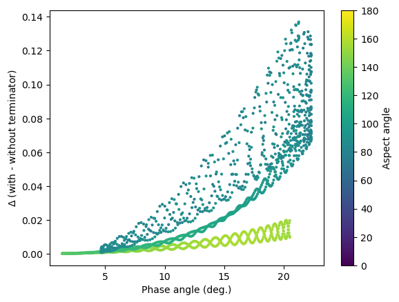
The difference between the two models is larger at larger phase angles, as expected. It is also larger for equatorial views, when the apparent shape varies the most.
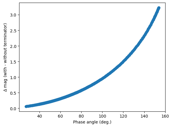
Effect of terminator: high phase angles
To understand better the difference between Ellipsoidal and EllipsoidalWithTerminator, let’s generate a SORCHA lightcurve for an asteroid that reach very high phase angle, (594913) ‘Aylo’chaxnim. We will set its shape to a perfect sphere to see the effect of the terminator only (i.e., all paraemters are going to be arbitrary).
[ ]:
# Target
sso = 594913
H = 16.2
ra0 = 180.0
dec0 = 0.0
period = 1.0
G1 = 0.62
G2 = 0.14
a_b = 1.0
a_c = 1.0
[18]:
# Choice of time frame
jd0 = 2461131.5  # Start date: here set to 2026-04-01
nbd = 600  # Number of epochs
step = 0.3  # Time step between epochs (days)

# Generate ephemerides
eph = ephemcc(
    sso,
    ep=jd0,
    nbd=nbd,
    step=step,
    tcoor=5,
    observer="X05",
    output="-- iofile(ephemcc-photom.xml),--lighttime",
)
[ ]:
# Build the observations dataframe
observations_df = pd.DataFrame(
    {
        "fieldMJD_TAI": eph.Date.values,
        "H_filter": H * np.ones(nbd),
        "G1": G1 * np.ones(nbd),
        "G2": G2 * np.ones(nbd),
        "RA_deg": eph.RA.values,
        "Dec_deg": eph.DEC.values,
        "RA_s_deg": eph.RA_h.values,
        "Dec_s_deg": eph.DEC_h.values,
        "Period": period * np.ones(nbd),
        "Time0": jd0 * np.ones(nbd),
        "phi0": np.radians(0) * np.ones(nbd),
        "RA0": np.radians(ra0) * np.ones(nbd),
        "Dec0": np.radians(dec0) * np.ones(nbd),
        "Period": period * np.ones(nbd),
        "a/b": a_b * np.ones(nbd),
        "a/c": a_c * np.ones(nbd),
        "Range_LTC_km": eph.Dobs.values * au,
        "Obj_Sun_LTC_km": eph.Dhelio.values * au,
        "phase_deg": eph.Phase.values,
    }
)

# Compute magnitude: base, ellipsoidal, ellipsoidal with terminator
observations_df = PPCalculateApparentMagnitudeInFilter(observations_df.copy(), "HG1G2", "r", "HG1G2_mag")

observations_df = PPCalculateApparentMagnitudeInFilter(
    observations_df.copy(), "HG1G2", "r", "LC_HG1G2_mag", "ellipsoidal"
)

observations_df = PPCalculateApparentMagnitudeInFilter(
    observations_df.copy(), "HG1G2", "r", "LCwT_HG1G2_mag", "ellipsoidalwithterminator"
)
[ ]:
fig, ax = plt.subplots(1, 2, figsize=(10, 5), sharey=True, gridspec_kw={"wspace": 0})

# --------------------------------------------------------------------------------
# Apparent magnitude vs time
ax[0].plot(
    observations_df["fieldMJD_TAI"],
    observations_df["HG1G2_mag"],
    linestyle="--",
    color="C0",
    label="HG1G2 baseline",
)
ax[0].plot(
    observations_df["fieldMJD_TAI"],
    observations_df["LC_HG1G2_mag"],
    linestyle="-",
    color="C1",
    label="With lightcurve",
)
ax[0].plot(
    observations_df["fieldMJD_TAI"],
    observations_df["LCwT_HG1G2_mag"],
    linestyle="dotted",
    color="C1",
    label="With lightcurve and terminator",
)

# --------------------------------------------------------------------------------
# Apparent magnitude vs phase
ax[1].plot(
    observations_df["phase_deg"],
    observations_df["HG1G2_mag"],
    linestyle="--",
    color="C0",
    label="HG1G2 baseline",
)
ax[1].plot(
    observations_df["phase_deg"],
    observations_df["LC_HG1G2_mag"],
    linestyle="-",
    color="C1",
    label="With lightcurve",
)
ax[1].plot(
    observations_df["phase_deg"],
    observations_df["LCwT_HG1G2_mag"],
    linestyle="dotted",
    color="C2",
    label="With lightcurve and terminator",
)

# --------------------------------------------------------------------------------
# Axes
for a in ax:
    a.legend()
    a.grid()
ax[0].set_xlabel("Time since first observation (days)")
ax[1].set_xlabel("Phase angle (degrees)")
ax[0].set_ylabel("Apparent magnitude")
ax[0].invert_yaxis()

fig.tight_layout()
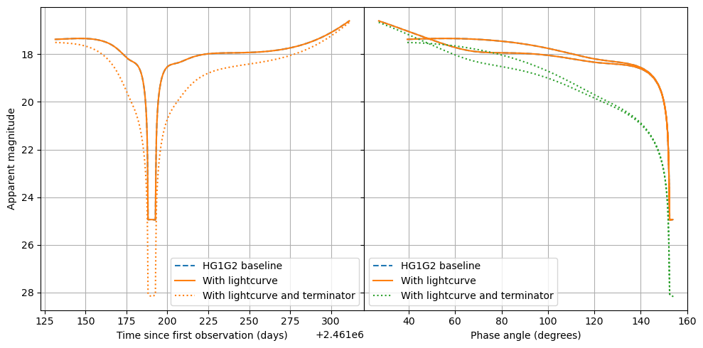
The Ellipsoidal model here above is strictly equal to the HG1G2 solution, because we forced the shape to be a sphere. The EllipsoidalWithTerminator solution, however, strongly diverges as the phase angle increases because the fraction of illuminated surface decreases.
Let’s finally see this difference between the two Ellispoidal models:
[ ]:
fig, ax = plt.subplots()

# Plot the difference between lightcurve with and without terminator
ax.scatter(
    observations_df["phase_deg"],
    observations_df["LCwT_HG1G2_mag"] - observations_df["LC_HG1G2_mag"],
    linestyle="-",
)

# Axes
ax.set_xlabel("Phase angle (deg.)")
ax.set_ylabel(r"$\Delta$ mag (with - without terminator)")