Realistic lightcurves of ellipsoids

This notebook demonstrates how to generate lightcurves within sorcha, under the assumption that the Solar System Objects (SSOs) are simple tri-axial ellipsoids, defined by $ a \ge `b :nbsphinx-math:ge `c$, in simple short-axis rotation mode.

[1]:

import numpy as np
import pandas as pd

import rocks
import requests

import astropy.units as u
from astropy.coordinates import SkyCoord

from sorcha.modules.PPCalculateApparentMagnitudeInFilter import (
    PPCalculateApparentMagnitudeInFilter,
)

import matplotlib.pyplot as plt

# Constant
au = 1.495978707e8  # AU in km

/home/bcarry/anaconda3/envs/sorcha/lib/python3.11/site-packages/assist/__init__.py:44: UserWarning: pkg_resources is deprecated as an API. See https://setuptools.pypa.io/en/latest/pkg_resources.html. The pkg_resources package is slated for removal as early as 2025-11-30. Refrain from using this package or pin to Setuptools<81.
  import pkg_resources

Lightweight ephemeris function

We will need to compute ephemerides, so let’s query the Miriade Virtual Observatory Web service.

[2]:

def ephemcc(ident, ep, nbd=None, step=None, observer="500", rplane="1", tcoor=5):
    """Gets asteroid ephemerides from IMCCE Miriade for a suite of JD for a single SSO
    Original function by M. Mahlke

    :ident: int, float, str - asteroid identifier
    :ep: float, str, list - Epoch of computation
    :observer: str - IAU Obs code - default to geocenter: https://minorplanetcenter.net//iau/lists/ObsCodesF.html
    :returns: pd.DataFrame - Input dataframe with ephemerides columns appended
              False - If query failed somehow

    """

    # ------
    # Miriade URL
    url = "https://ssp.imcce.fr/webservices/miriade/api/ephemcc.php"

    # Query parameters
    params = {
        "-name": f"{ident}",
        "-mime": "json",
        "-rplane": rplane,
        "-tcoor": tcoor,
        "-output": "--jd",
        "-observer": observer,
        "-tscale": "UTC",
    }

    # Single epoch of computation
    if type(ep) != list:
        # Set parameters
        params["-ep"] = ep
        if nbd != None:
            params["-nbd"] = nbd
        if step != None:
            params["-step"] = step

        # Execute query
        try:
            r = requests.post(url, params=params, timeout=80)
        except requests.exceptions.ReadTimeout:
            return False

    # Multiple epochs of computation
    else:
        # Epochs of computation
        files = {"epochs": ("epochs", "\n".join(["%.6f" % epoch for epoch in ep]))}

        # Execute query
        try:
            r = requests.post(url, params=params, files=files, timeout=50)
        except requests.exceptions.ReadTimeout:
            return False

    j = r.json()

    # Read JSON response
    try:
        ephem = pd.DataFrame.from_dict(j["data"])
    except KeyError:
        return False

    return ephem

Definition of simulation

We first define the epochs of the simulation: starting date (expressed in JD), the number of epochs to simulate, and time step between each (in days).

[3]:

# Choice of time frame
jd0 = 2461041.5 # Start date: here set to 2026-01-01
nbd = 1500 # Number of epochs
step = 0.3 # Time step between epochs (days)

We then define the target. It can be an asteroid name/designation or number. The absolute magnitude and spin properties (coordinates and period) are then retrieved from SsODNet (see Berthier et al., 2023). Alternatively, you can define all parameters by hand:

H the absolute magnitude
ra0 the right ascension of the spin coordinates (equatorial frame, in degrees)
dec0 the declination of the spin coordinates (equatorial frame, in degrees)
period the sidereal rotation period (in hour)
G1 and G2 the phase curve coefficients
a_b the ratio of equatorial diameters (a and b)
a_c the ratio between the longest (equatorial) diameter (a) and the polar diameter (c)

[4]:

# Target
sso = 22

# Retrieve the target properties from SsODNet
sc = rocks.Rock(sso)
H = sc.H.value
ra0 = sc.spin.RA0.value
dec0 = sc.spin.DEC0.value
period = sc.spin.period.value[0] / 24.0

# Arbitrary phase function and shape
G1 = 0.62
G2 = 0.14
a_b = 1.5
a_c = 2.0

[5]:

# Generate ephemerides
eph = ephemcc(sso, ep=jd0, nbd=nbd, step=step, tcoor=5, observer='X05')

[6]:

# Build the observations dataframe
observations_df = pd.DataFrame(
    {
        "fieldMJD_TAI": eph.Date.values,
        "H_filter": H * np.ones(nbd),
        "G1": G1 * np.ones(nbd),
        "G2": G2 * np.ones(nbd),
        "RA_deg": eph.RA.values,
        "Dec_deg": eph.DEC.values,
        "Period": period * np.ones(nbd),
        "Time0": jd0 * np.ones(nbd),
        "phi0": np.radians(0) * np.ones(nbd),
        "RA0": np.radians(ra0) * np.ones(nbd),
        "Dec0": np.radians(dec0) * np.ones(nbd),
        "Period": period * np.ones(nbd),
        "a/b": a_b * np.ones(nbd),
        "a/c": a_c * np.ones(nbd),
        "Range_LTC_km": eph.Dobs.values * au,
        "Obj_Sun_LTC_km": eph.Dhelio.values * au,
        "phase_deg": eph.Phase.values,
    }
)

observations_df

[6]:

	fieldMJD_TAI	H_filter	G1	G2	RA_deg	Dec_deg	Period	Time0	phi0	RA0	Dec0	a/b	a/c	Range_LTC_km	Obj_Sun_LTC_km	phase_deg
0	2461041.5	6.79	0.62	0.14	359.334334	-11.523769	0.172842	2461041.5	0.0	3.405137	-0.049463	1.5	2.0	4.177865e+08	4.049300e+08	20.522908
1	2461041.8	6.79	0.62	0.14	359.407445	-11.465113	0.172842	2461041.5	0.0	3.405137	-0.049463	1.5	2.0	4.183388e+08	4.048958e+08	20.502883
2	2461042.1	6.79	0.62	0.14	359.482166	-11.406700	0.172842	2461041.5	0.0	3.405137	-0.049463	1.5	2.0	4.188799e+08	4.048617e+08	20.481478
3	2461042.4	6.79	0.62	0.14	359.555298	-11.348389	0.172842	2461041.5	0.0	3.405137	-0.049463	1.5	2.0	4.194149e+08	4.048277e+08	20.461570
4	2461042.7	6.79	0.62	0.14	359.628519	-11.289645	0.172842	2461041.5	0.0	3.405137	-0.049463	1.5	2.0	4.199635e+08	4.047937e+08	20.441432
...	...	...	...	...	...	...	...	...	...	...	...	...	...	...	...	...
1495	2461490.0	6.79	0.62	0.14	100.442283	35.559274	0.172842	2461041.5	0.0	3.405137	-0.049463	1.5	2.0	3.696081e+08	4.089152e+08	21.330520
1496	2461490.3	6.79	0.62	0.14	100.514005	35.545997	0.172842	2461041.5	0.0	3.405137	-0.049463	1.5	2.0	3.702196e+08	4.089530e+08	21.336566
1497	2461490.6	6.79	0.62	0.14	100.583783	35.532027	0.172842	2461041.5	0.0	3.405137	-0.049463	1.5	2.0	3.708370e+08	4.089908e+08	21.344123
1498	2461490.9	6.79	0.62	0.14	100.656047	35.517137	0.172842	2461041.5	0.0	3.405137	-0.049463	1.5	2.0	3.714625e+08	4.090287e+08	21.349582
1499	2461491.2	6.79	0.62	0.14	100.729880	35.503386	0.172842	2461041.5	0.0	3.405137	-0.049463	1.5	2.0	3.720775e+08	4.090665e+08	21.353868

1500 rows × 16 columns

SORCHA simulation

We first simply compute the apparent magnitude, using the $H G_1 G_2$ formalism, as a baseline.

[7]:

observations_df = PPCalculateApparentMagnitudeInFilter(observations_df.copy(), "HG1G2", "r", "HG1G2_mag")

We then load the lightcurve methods of SORCHA add-ons:

[8]:

from sorcha.lightcurves.lightcurve_registration import LC_METHODS, update_lc_subclasses
update_lc_subclasses()
print('Lightcurve methods: ' + ', '.join(LC_METHODS))

Lightcurve methods: identity, sinusoidal, ellipsoidal, ellipsoidalwithterminator

We can now compute the apparent magnitude with the lightcurve effect (using the $H G_1 G_2$ formalism for consistency).

[9]:

observations_df = PPCalculateApparentMagnitudeInFilter(
    observations_df.copy(), "HG1G2", "r", "LC_HG1G2_mag", "ellipsoidal"
)

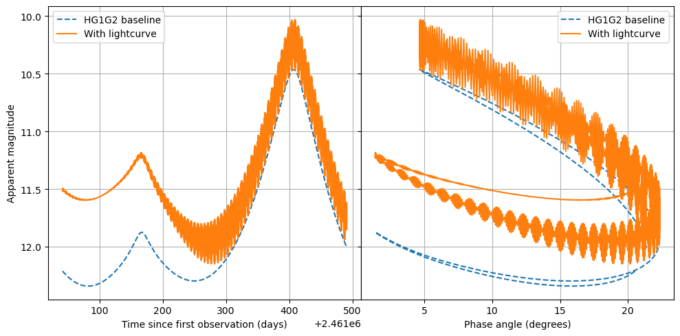
Graphics illustrating the lightcurve effect

[10]:

fig, ax = plt.subplots(1, 2, figsize=(10, 5), sharey=True, gridspec_kw={"wspace": 0})

# --------------------------------------------------------------------------------
# Apparent magnitude vs time
ax[0].plot(
    observations_df["fieldMJD_TAI"],
    observations_df["HG1G2_mag"],
    linestyle="--",
    color="C0",
    label="HG1G2 baseline",
)
ax[0].plot(
    observations_df["fieldMJD_TAI"],
    observations_df["LC_HG1G2_mag"],
    linestyle="-",
    color="C1",
    label="With lightcurve",
)

# --------------------------------------------------------------------------------
# Apparent magnitude vs phase
ax[1].plot(
    observations_df["phase_deg"],
    observations_df["HG1G2_mag"],
    linestyle="--",
    color="C0",
    label="HG1G2 baseline",
)
ax[1].plot(
    observations_df["phase_deg"],
    observations_df["LC_HG1G2_mag"],
    linestyle="-",
    color="C1",
    label="With lightcurve",
)

# --------------------------------------------------------------------------------
# Axes
for a in ax:
    a.legend()
    a.grid()
ax[0].set_xlabel("Time since first observation (days)")
ax[1].set_xlabel("Phase angle (degrees)")
ax[0].set_ylabel("Apparent magnitude")
ax[0].invert_yaxis()

fig.tight_layout()
fig.savefig("ellipsoidal_lightcurve_example.png", dpi=300)

../../../_images/notebooks_lightcurve_ellipsoidal_demo_Ellipsoidal_Lightcurve_17_0.png